Supervised learning involves training a model on labeled data. In the context of consumer complaints, supervised learning techniques can be applied to predict important outcomes, such as sentiment scores or complaint categories, based on various features. By utilizing labeled data, we can build models that help organizations like the CFPB or financial companies to automate the decision-making process, prioritize complaints, and improve overall complaint resolution strategies.
Import packages and load the dataset
# Import necessary packagesimport pandas as pdimport numpy as npimport matplotlib.pyplot as plt# Load the datasetdf = pd.read_csv("../../data/processed-data/complaints.csv")df.head()
Regression analysis is used to predict continuous outcomes based on independent variables. In this context, we applied regression techniques to predict the sentiment score of a complaint based on features such as product type, issue, and complaint tags. By understanding the relationship between these features and sentiment scores, financial institutions or the CFPB can better measure the emotional tone of complaints and determine their urgency or priority for resolution. A regression model can help automate the process of assessing complaints, ensuring that companies respond appropriately based on the predicted sentiment.
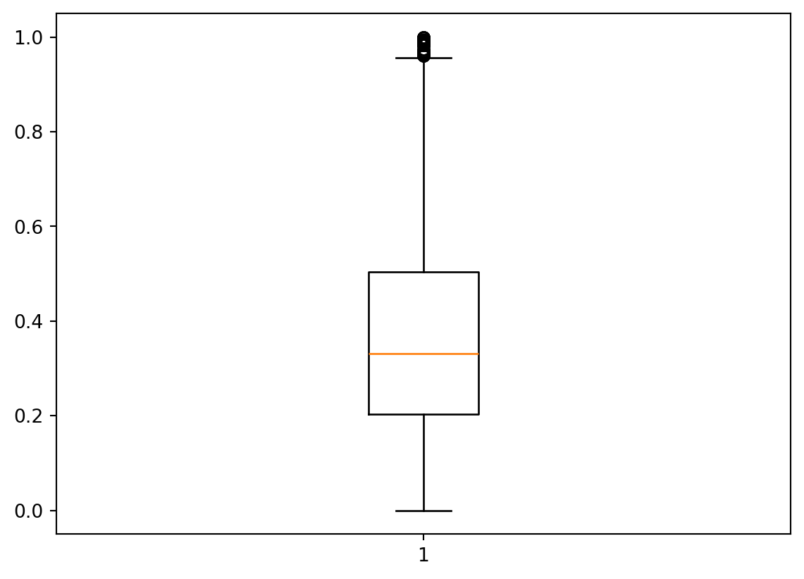
Since complaints are typically negative, we used the negative score (after applying min-max rescaling) as the predictor. The negative score ranges from 0 to 1, with higher values indicating stronger negative sentiment. From the boxplot of the negative scores, we observe that the majority of scores are centered between 0.2 and 0.5, indicating moderate negative sentiment. This suggests that most complaints, while negative, do not represent extreme dissatisfaction, and may require more advanced handling by companies to improve customer experience.
plt.boxplot(df['negative-score'])
{'whiskers': [<matplotlib.lines.Line2D at 0x125b59b90>,
  <matplotlib.lines.Line2D at 0x125b5a790>],
 'caps': [<matplotlib.lines.Line2D at 0x125b5b550>,
  <matplotlib.lines.Line2D at 0x125b641d0>],
 'boxes': [<matplotlib.lines.Line2D at 0x104f10c10>],
 'medians': [<matplotlib.lines.Line2D at 0x125b64d10>],
 'fliers': [<matplotlib.lines.Line2D at 0x125b65810>],
 'means': []}
Regression Model Implementation
In this section, we apply multiple regression methods to predict the negative sentiment score of complaints based on various features. The process follows these steps:
Data Preprocessing:
Irrelevant columns such as Complaint_ID, Complaint, Tags, and others are dropped to ensure only relevant predictors are used.
The target variable, negative-score, is selected as the output for prediction.
One-Hot Encoding:
Categorical features are encoded using one-hot encoding, converting categorical variables into a format suitable for machine learning models. We use the pd.get_dummies method with the drop_first=True parameter to avoid multicollinearity.
Train-Test Split:
The dataset is split into training and testing sets with 80% of the data used for training and 20% for testing. The split is done using train_test_split, with a random state set for reproducibility.
Model Training:
Linear regression
Decision trees regression
Random forest regression
Gradient boosting regression
Evaluation:
The model’s performance is evaluated using two metrics: Mean Squared Error (MSE) and Mean Absolute Error (MAE). These metrics provide insights into the prediction accuracy.
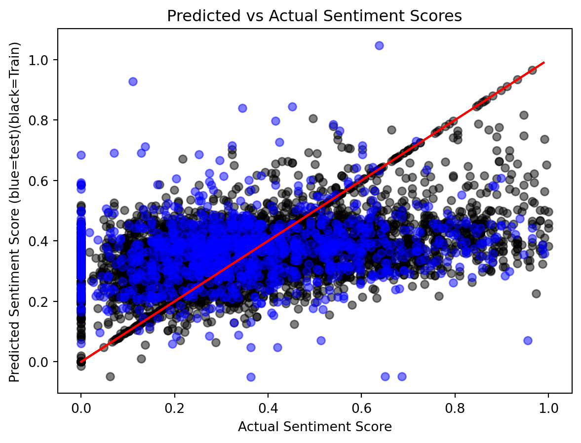
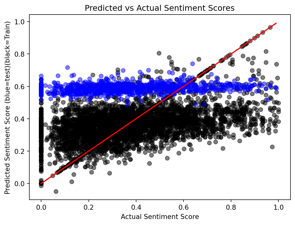
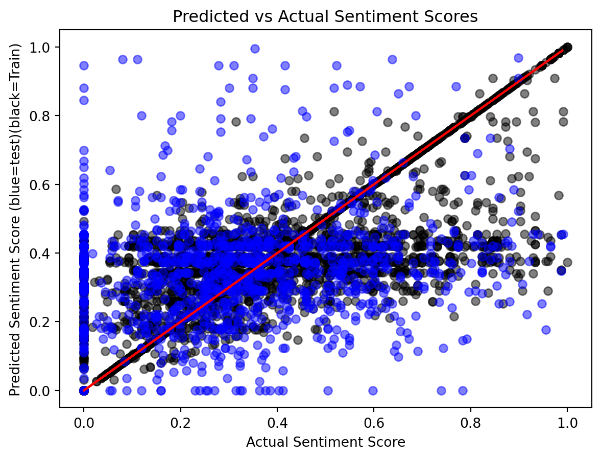
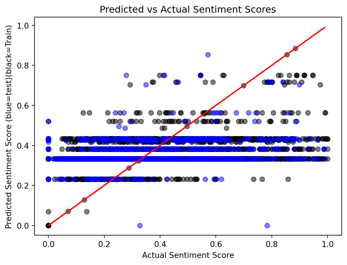
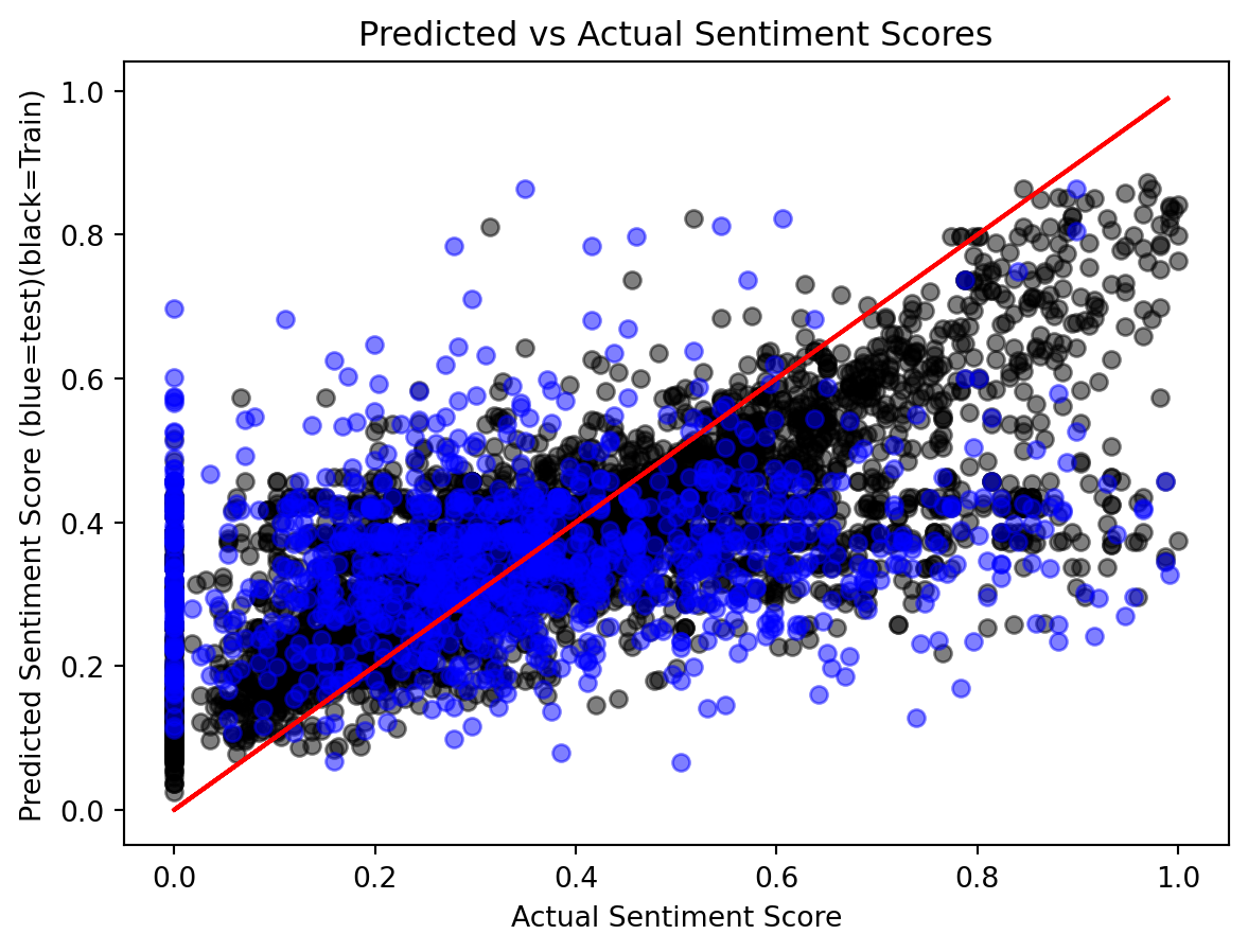
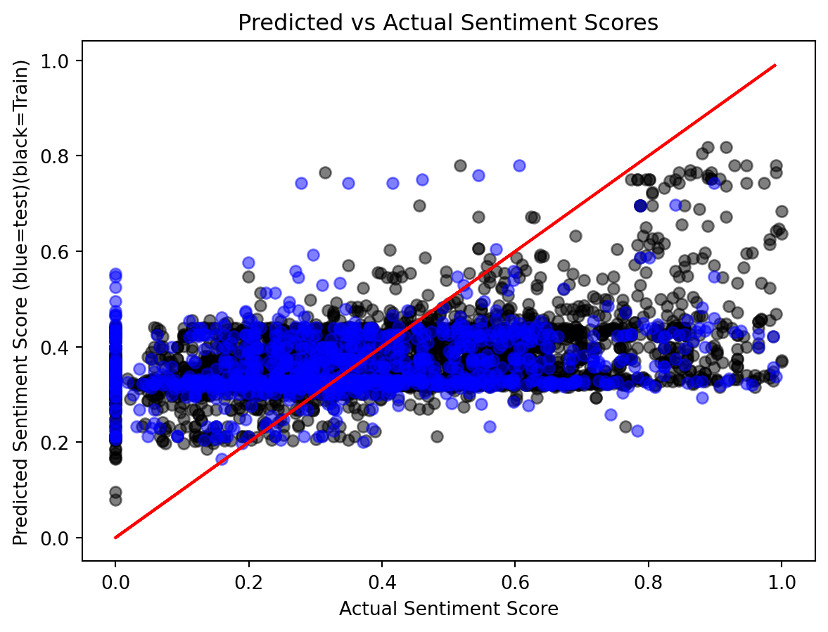
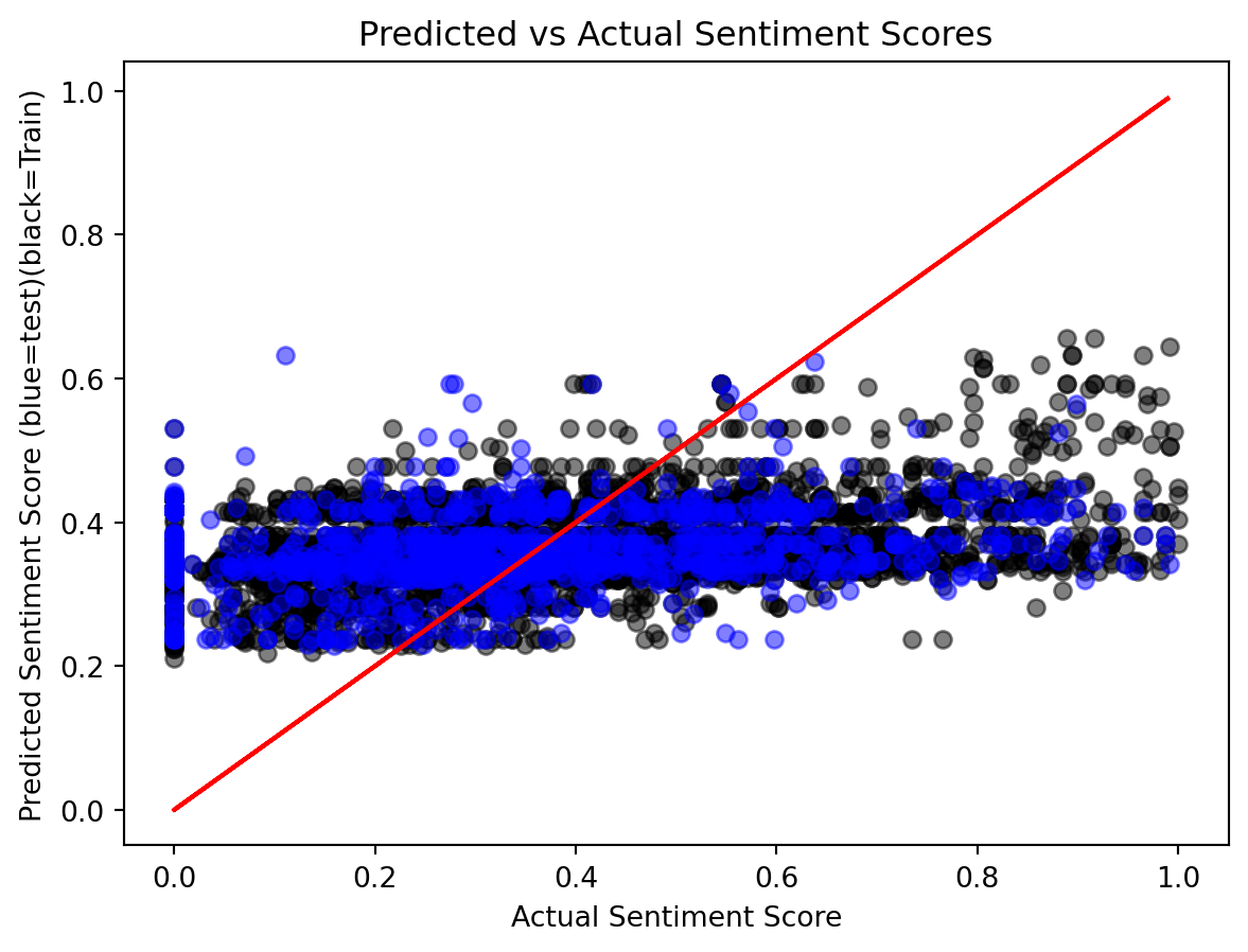
A parity plot is used to visualize the actual vs. predicted sentiment scores. The plot differentiates between the training and test data, with the actual sentiment scores shown against the predicted values. The red line represents the perfect parity, where the predicted values exactly match the actual ones.
By evaluating the model with these metrics and visualizations, we can assess the quality of the regression model in predicting sentiment scores based on the features provided.
from sklearn.linear_model import LinearRegressionfrom sklearn.model_selection import train_test_splitfrom sklearn.metrics import mean_squared_error, mean_absolute_error# Drop irrelevant columnsX = df.drop(columns=['Complaint_ID', 'sentiment_score', 'Complaint', 'Tags', 'Date', 'Company Response', 'Company Public Response', 'cleaned_complaints','negative-score', 'Clean Complaint Length', 'Category'])print(X.columns)# Rescale the sentiment scorey = df['negative-score']# One-Hot Encoding for categorical columnscategorical_cols = X.select_dtypes(include=['object']).columnsX_encoded = pd.get_dummies(X, columns=categorical_cols, drop_first=True)# Split data into train and test setsX_train, X_test, y_train, y_test = train_test_split(X_encoded, y, test_size=0.2, random_state=50)# Evaluation function for regressiondef reg_evaluation(y_train, yp_train, y_test, yp_test):print("Mean Squared Error (MSE):", mean_squared_error(y_test, yp_test))print("Mean Absolute Error (MAE):", mean_absolute_error(y_test, yp_test))# Parity plot plt.plot(y_train, yp_train,"o", color='black', alpha=0.5) plt.plot(y_test, yp_test, "o", color='blue', alpha=0.5) plt.plot(y_test, y_test, "-", color='r') plt.xlabel('Actual Sentiment Score') plt.ylabel('Predicted Sentiment Score (blue=test)(black=Train)') plt.title('Predicted vs Actual Sentiment Scores') plt.show()
Linear regression is a simple model that assumes a linear relationship between the input features and the target variable. In the context of this analysis, linear regression is used as a benchmark model to predict the negative sentiment score of complaints based on features such as product type, issue, and other complaint-related attributes.
# Fit the modelmodel = LinearRegression()model.fit(X_train, y_train)# Predictions and evaluationyp_train = model.predict(X_train)yp_test = model.predict(X_test)print("R-squared:", model.score(X_test, y_test))reg_evaluation(y_train, yp_train, y_test, yp_test)
R-squared: -0.04569164578055629
Mean Squared Error (MSE): 0.05174344651543658
Mean Absolute Error (MAE): 0.1793583736941442
The results of the linear regression model indicate poor performance on both the training and test datasets. Most of the predicted values are clustered around 0, with one test prediction even reaching -1.25. Since the sentiment score is expected to range between 0 and 1, these results demonstrate that linear regression is not suitable for predicting values constrained within a specific range.
Mean Squared Error (MSE): 0.10767365547804099
Mean Absolute Error (MAE): 0.28354329553660157
To further evaluate the predictive capability of the linear model, we applied a sigmoid function to rescale the predictions to the range [0, 1]. After this transformation, the model’s performance improved, with significant reductions in both Mean Squared Error (MSE) and Mean Absolute Error (MAE). However, the model still showed poor training results, with most predictions for the training data clustering between 0.2 and 0.5 rather than closely aligning with the ideal red line. Similarly, test predictions were confined to a narrow range of 0.5 to 0.6. These findings suggest that while the sigmoid transformation provides some improvement, advanced models are needed to achieve better prediction accuracy.
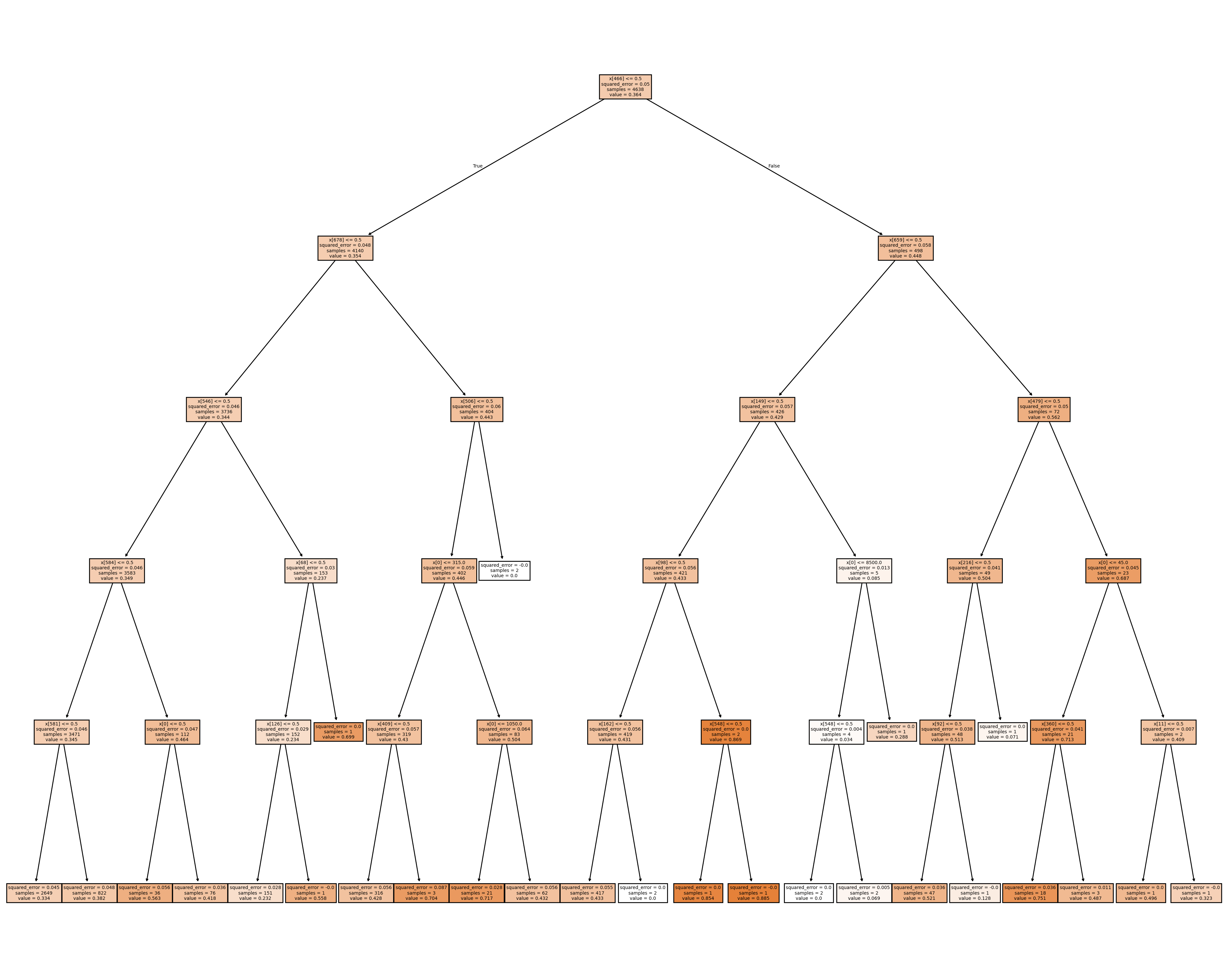
Decision Tree Regression
Decision Tree Regression uses a tree-like structure to make predictions. The model recursively splits the data into subsets based on feature values that maximize the reduction in variance at each step. At each node of the tree, a decision is made to divide the data into smaller groups, which ultimately leads to predictions at the leaf nodes.
One of the primary advantages of decision trees is their ability to capture non-linear relationships between features and the target variable. Unlike linear regression, which assumes a linear relationship, decision trees can model more complex interactions within the data. They are also highly interpretable, as the splitting rules provide a clear explanation of the decision-making process.
Initial Decision Tree Regression (Default Hyperparameters)
from sklearn.tree import DecisionTreeRegressorfrom sklearn.ensemble import RandomForestRegressor# Fit the modelmodel = DecisionTreeRegressor()model.fit(X_train, y_train)# Predictions and evaluationyp_train = model.predict(X_train)yp_test = model.predict(X_test)reg_evaluation(y_train, yp_train, y_test, yp_test)
Mean Squared Error (MSE): 0.06418484717262822
Mean Absolute Error (MAE): 0.19540570820429543
The results from the decision tree regression are significantly better than those of the linear regression model with the sigmoid transformation. More data points for both the training and test sets are closer to the ideal red line, with an MSE of 0.06 compared to 0.11 and an MAE of 0.19 compared to 0.28.
However, decision trees are prone to overfitting, especially when the tree grows too deep. Overfitting can cause the model to memorize training data rather than generalize to new, unseen data. To mitigate this issue, hyperparameters such as max_depth, min_samples_split, and min_samples_leaf can be tuned to balance model accuracy and consistency.
To ensure optimal performance, we perform hyperparameter tuning to identify the best tree depth. This allows the model to achieve a good fit while maintaining its ability to generalize to new data.
Hyperparameter Tuning (max_depth)
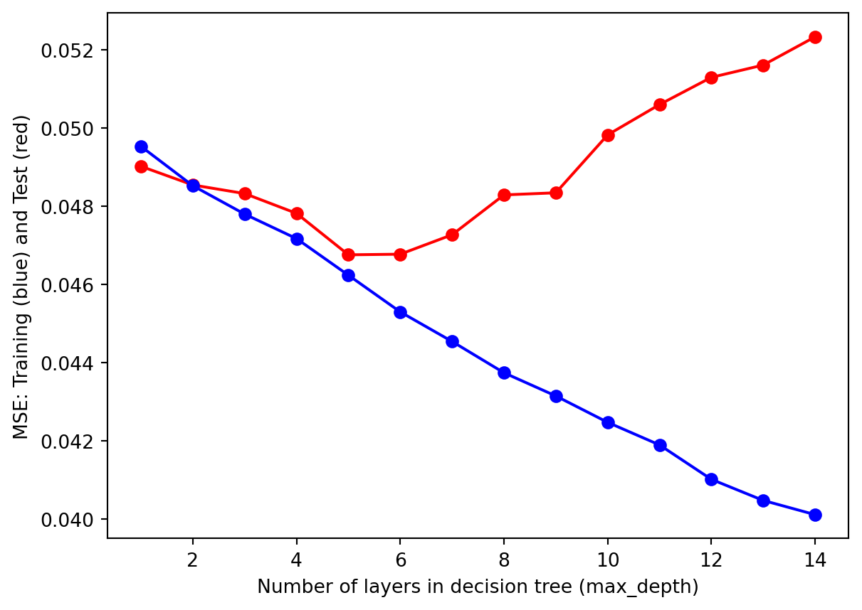
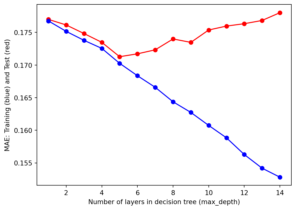
# Hyper-Parameter tuning (max_depth)def tuning_depth(tree): test_results=[] train_results=[]for num_layer inrange(1,15):if tree=="DecisionTreeRegression": model = DecisionTreeRegressor(max_depth=num_layer)if tree=="RandomForestRegressor": model = RandomForestRegressor(max_depth=num_layer) model = model.fit(X_train, y_train) yp_train=model.predict(X_train) yp_test=model.predict(X_test) test_results.append([num_layer,mean_squared_error(y_test, yp_test),mean_absolute_error(y_test, yp_test)]) train_results.append([num_layer,mean_squared_error(y_train, yp_train),mean_absolute_error(y_train, yp_train)]) test_results = np.array(test_results) train_results = np.array(train_results)return test_results, train_resultsdef plot_result(i, j, xlab, ylab, test_results, train_results): plt.plot(test_results[:,i], test_results[:,j], '-or') plt.plot(train_results[:,i], train_results[:,j], '-ob') plt.xlabel(xlab) plt.ylabel(ylab) plt.show()test_results, train_results = tuning_depth("DecisionTreeRegression")plot_result(0, 1, "Number of layers in decision tree (max_depth)", "MSE: Training (blue) and Test (red)", test_results, train_results)plot_result(0, 2, "Number of layers in decision tree (max_depth)", "MAE: Training (blue) and Test (red)", test_results, train_results)
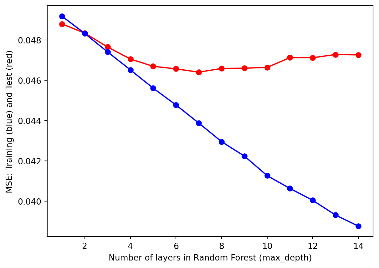
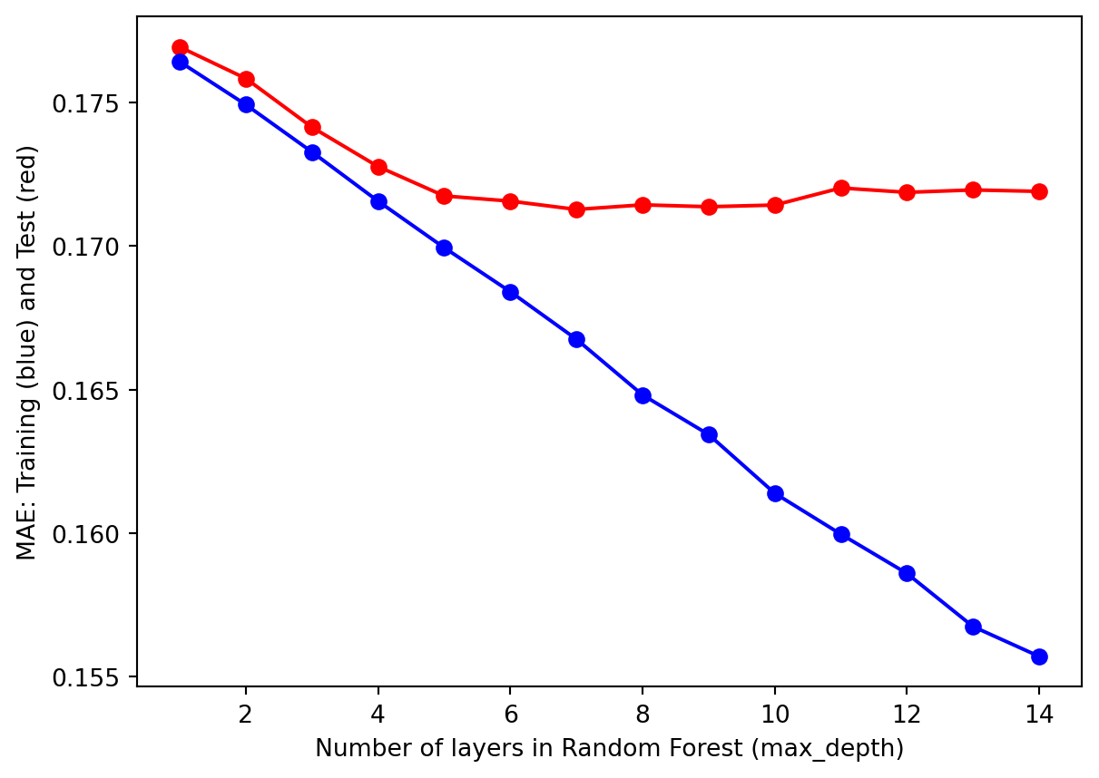
From the hyperparameter tuning results, we observe similar trends for both the Mean Squared Error and Mean Absolute Error criteria. As the number of layers (i.e., max_depth) increases, the model becomes better at learning the training data, reflected by a steady decrease in MSE and MAE for the training set. However, the performance on the test set exhibits a U-shaped pattern: the error decreases initially, reaches a minimum at max_depth = 5, and then starts to increase.
This pattern indicates that with a max_depth smaller than 5, the model underfits the data and fail to capture underlying patterns, resulting in model inaccuracy and high errors. In contrast, as the max_depth exceeds 5, the model starts to overfit, memorizing training data instead of generalizing to unseen test data. Overfitting leads to deteriorating performance on the test set despite continued improvement on the training set.
The results suggest that the optimal max_depth for the decision tree is 5. At this depth, the model finds the best balance between fitting the training data and maintaining generalization ability for the test data, ensuring both accuracy and consistency. This demonstrates the importance of hyperparameter tuning in achieving a model that performs well across different datasets.
Optimized Decision Tree Model (max_depth=5)
# Fit the modelmodel_opt = DecisionTreeRegressor(max_depth=5)model_opt.fit(X_train, y_train)# Predictions and evaluationyp_train = model_opt.predict(X_train)yp_test = model_opt.predict(X_test)reg_evaluation(y_train, yp_train, y_test, yp_test)
Mean Squared Error (MSE): 0.04673965626351558
Mean Absolute Error (MAE): 0.17125067975696856
Random Forest is an ensemble learning method that builds multiple decision trees and combines their outputs to improve prediction accuracy. By aggregating the predictions of individual trees, Random Forest reduces variance and mitigates overfitting.
Each tree in the Random Forest is trained on a random subset of the data using bootstrapping, where samples are drawn randomly with replacement. Additionally, the model introduces randomness at the feature level by selecting a random subset of features for each split in a tree. These mechanisms ensure the trees are uncorrelated, making the ensemble more robust.
In this context, Random Forest Regression helps predict sentiment scores by leveraging patterns across multiple features. This approach offers a more comprehensive view of the data compared to single models like linear regression or decision tree regression. Through ensemble learning, we aim to achieve higher accuracy and better generalization to unseen data.
Initial Random Forest Regression (Default Hyperparameters)
# Fit the modelmodel = RandomForestRegressor()model.fit(X_train, y_train)# Predictions and evaluationyp_train = model.predict(X_train)yp_test = model.predict(X_test)reg_evaluation(y_train, yp_train, y_test, yp_test)
Mean Squared Error (MSE): 0.05110149409520344
Mean Absolute Error (MAE): 0.17709374478600912
The prediction trends for both the training and test data are similar, with both sets of predictions closely following the ideal red line. This suggests that the model is capturing the general pattern of the data well. However, we observe that the predictions for the training data, particularly those with larger sentiment scores, perform better than the test data. This discrepancy indicates that while the model is fitting well to the training data, it may not be generalizing as effectively to unseen data, which is a common indication of overfitting.
The Mean Squared Error (MSE) and Mean Absolute Error (MAE) for the random forest model with default parameters are comparable to the results from the optimized single decision tree model, with the random forest model achieving an MSE of 0.05 and a MAE of 0.17. Given that random forests rely on aggregating multiple decision trees, they have the potential to improve further with proper tuning.
To achieve better performance, we need to explore hyperparameter tuning for the random forest model. By adjusting the parameter max_depth the maximum depth of the trees, we can optimize the model to better capture the underlying patterns in the data and improve its generalization to unseen test data.
Hyperparameter Tuning (max_depth)
test_results, train_results = tuning_depth("RandomForestRegressor")plot_result(0, 1, "Number of layers in Random Forest (max_depth)", "MSE: Training (blue) and Test (red)", test_results, train_results)plot_result(0, 2, "Number of layers in Random Forest (max_depth)", "MAE: Training (blue) and Test (red)", test_results, train_results)
As with the tuning results for the Decision Tree model, the Random Forest model also exhibits an optimal performance when the max_depth is set to 5. In this case, the error for the test data reaches its minimum at this depth. By setting the max_depth to 5, the Random Forest model is able to capture enough complexity in the data without becoming overly specific to the training set. This provides a better fit to the test data and ensures that the model performs well on unseen examples, which is crucial for effective prediction in real-world scenarios.
Optimized Random Forest Model (max_depth=5)
# Fit the modelmodel = RandomForestRegressor(max_depth=10)model.fit(X_train, y_train)# Predictions and evaluationyp_train = model.predict(X_train)yp_test = model.predict(X_test)reg_evaluation(y_train, yp_train, y_test, yp_test)
Mean Squared Error (MSE): 0.04671724652702078
Mean Absolute Error (MAE): 0.17126704748146343
Gradient Boosting Regression
Gradient boosting is another ensemble learning method that builds models sequentially. Unlike random forests, which create multiple independent trees and combine their predictions, gradient boosting focuses on improving the model’s performance. Each new model corrects the errors made by the previous one. This process continues until the model reaches a desired level of accuracy or a set number of iterations.
The key idea behind gradient boosting is to fit each new model to the residual errors (the difference between the actual and predicted values) of the previous model. This sequential learning process allows gradient boosting to capture complex relationships in the data that might be missed by simpler models like linear regression or decision trees.
One of the advantages of gradient boosting is that it can model both linear and non-linear relationships, making it suitable for a wide range of regression tasks. Another benefit of gradient boosting is that it often does not require hyperparameters tuing. While there are still important parameters, such as learning rate, number of estimators (trees), and tree depth, the model is generally more robust to hyperparameter variations and can still perform well even with default settings.
In the context of predicting sentiment scores, gradient boosting can help improve prediction accuracy by leveraging its ability to model complex relationships in the data.
from sklearn.ensemble import GradientBoostingRegressor# Fit the Gradient Boosting Regressor modelmodel = GradientBoostingRegressor()model.fit(X_train, y_train)# Predictions and evaluationyp_train = model.predict(X_train)yp_test = model.predict(X_test)reg_evaluation(y_train, yp_train, y_test, yp_test)
Mean Squared Error (MSE): 0.046281416947387355
Mean Absolute Error (MAE): 0.17149825120280854
Conclusion for Regression Analysis
Based on the regression results, we conclude that tree-based regression models outperform linear regression. Among all tree-based models, whether default or tuned, the performance of Decision Tree, Random Forest, and Gradient Boosting models is very similar. However, considering the variability in real-world data and the randomness in our train-test split, we select the Random Forest model as our final choice. It performs well on both training and test data, and as an ensemble model, it presents strong consistency across different datasets.
Classification
Classification techniques aim to categorize data into predefined classes or labels. For consumer complaints, classification models can be used to determine the category of a complaint based on features like the company involved, sentiment score, complaint amount, and narrative complaint length. This can help the CFPB or companies assess whether a complaint has been correctly categorized and identify potential misclassifications. By automating the classification process, organizations can streamline their complaint handling systems, ensuring complaints are routed to the appropriate department and addressed more efficiently.
Binary Classification
In this section, we apply multiple classification methods to predict the category of complaints based on various features. The process follows these steps:
Data Preprocessing:
Irrelevant columns such as Complaint_ID, Complaint, Tags, and others are dropped to ensure only relevant predictors are used.
The target variable, Category, is selected as the output for prediction.
For Binary Classification, the target variable indicates whether the complaint is related to Credit Reporting.
For Multiclass Classification, the target variable consists of the six categories of complaints.
One-Hot Encoding:
Categorical features are encoded using one-hot encoding, converting categorical variables into a format suitable for machine learning models. We use the pd.get_dummies method with the drop_first=True parameter to avoid multicollinearity.
Train-Test Split:
The dataset is split into training and testing sets with 80% of the data used for training and 20% for testing. The split is done using train_test_split, with a random state set for reproducibility.
Model Training:
Logistic regression
KNN classification
Random forest classification
Evaluation:
The model’s performance is evaluated using two metrics: Confusion Matrix and ROC Curve. These metrics provide insights into the prediction accuracy.
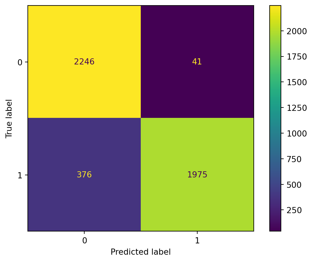
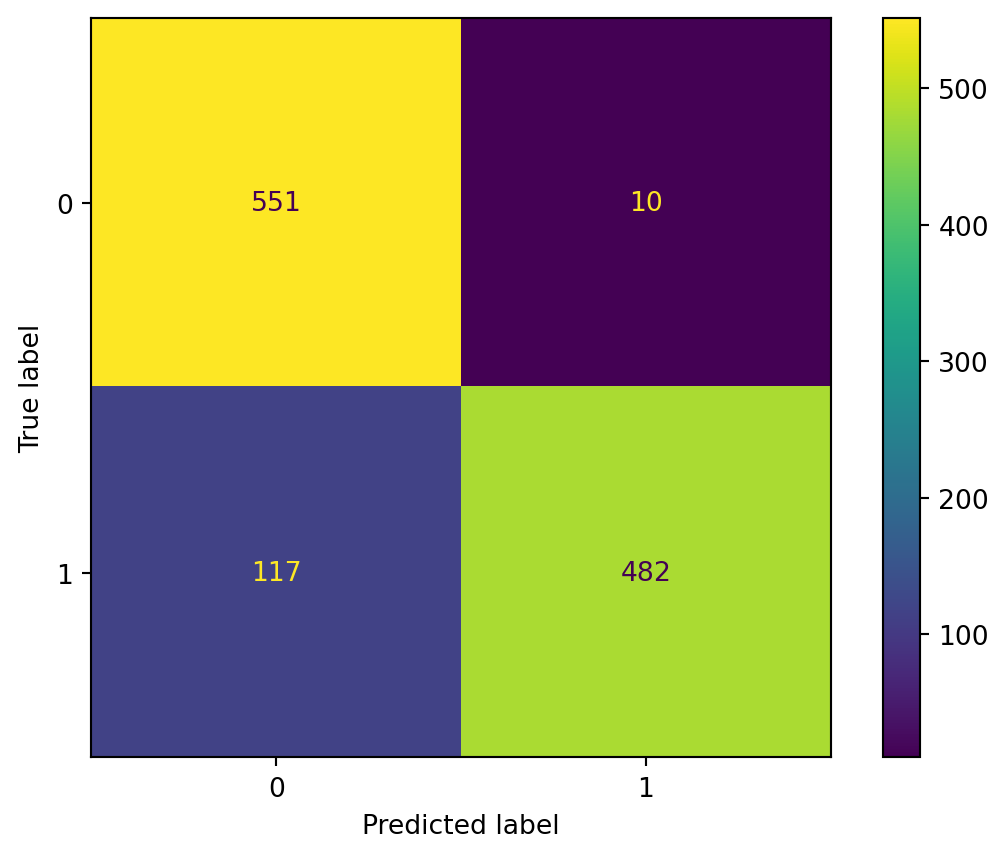
Confusion Matrix
The confusion matrix provides insight into the model’s classification performance by comparing the true labels to the predicted labels. It shows the number of true positives, true negatives, false positives, and false negatives.
We also calculate key metrics for both the positive and negative classes (Y=1 for positive, Y=0 for negative): Accuracy: The overall proportion of correctly classified instances. Recall: The ability of the model to correctly identify positive (or negative) instances. Precision: The accuracy of positive (or negative) predictions. F1 Score: The harmonic mean of precision and recall, providing a single metric to balance both.
ROC Curve
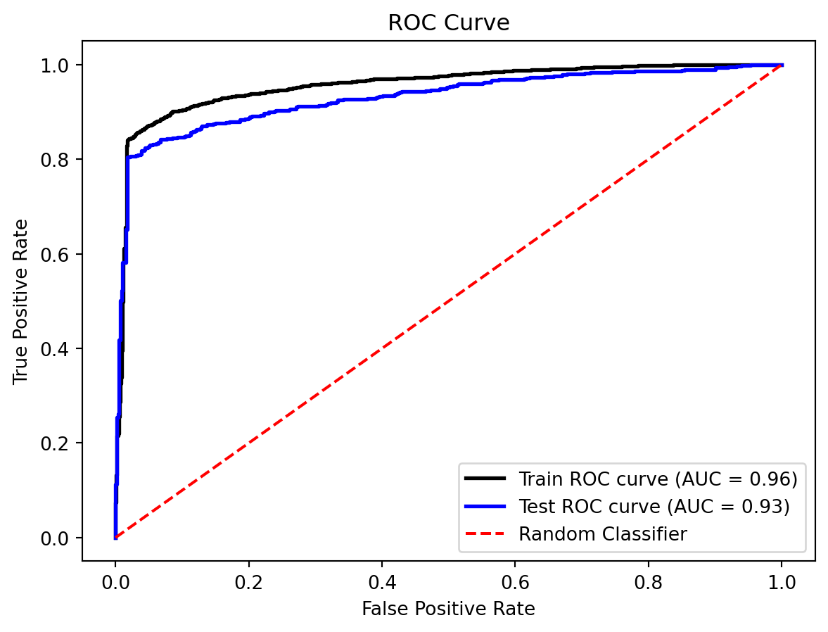
The Receiver Operating Characteristic (ROC) curve is used to evaluate the performance of a binary classifier. It plots the True Positive Rate (TPR) against the False Positive Rate (FPR) at various thresholds. The Area Under the Curve (AUC) is used to summarize the ROC curve. A higher AUC indicates a better performing model.
We plot the ROC curve for both the training and test datasets to compare the model’s performance across different data splits.
By evaluating the model with these metrics and visualizations, we can assess the quality of the classification model in predicting categories of complaints based on the features provided.
# Drop irrelevant columnsX = df.drop(columns=['Complaint_ID', 'Complaint', 'Tags', 'Product', 'Sub-product', 'Issue', 'Sub-issue','Date', 'Company Response', 'Company Public Response', 'cleaned_complaints','Category'])print(X.columns, end='\n\n')print(df['Category'].value_counts())y = (df['Category']=='Credit reporting').astype(int)# One-Hot Encoding for categorical columnscategorical_cols = X.select_dtypes(include=['object']).columnsX = pd.get_dummies(X, columns=categorical_cols, drop_first=True)# Split data into train and test setsX_train, X_test, y_train, y_test = train_test_split(X, y, test_size=0.2, random_state=50)
Logistic Regression is a statistical model that is commonly used for binary classification problems, though it can also be extended to multiclass classification. Despite its name, it is a linear model used to predict the probability that an instance belongs to a particular class.
In binary classification, the model predicts a binary outcome (0 or 1, representing two classes). It does this by calculating the weighted sum of the input features, and then passing the result through a logistic (sigmoid) function, which squashes the output into a value between 0 and 1. This value can be interpreted as the probability of the instance belonging to the positive class. The decision boundary is typically set at 0.5, meaning that if the predicted probability is greater than 0.5, the instance is classified as the positive class (1), and if it is less than 0.5, the instance is classified as the negative class (0).
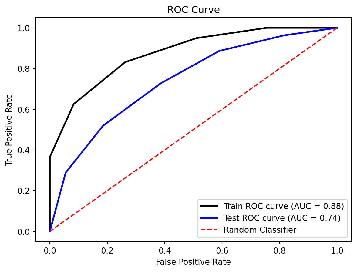
The predictions made by the Logistic Regression model are generally great, presenting both high accuracy and consistency. The accuracy score for the training data is 0.90, while the test data accuracy is 0.88. The similar performance on both training and test sets indicates that, despite some minor misclassifications, the model is not overfitting but rather has a stable and consistent performance across different datasets, which is a good sign of its ability to generalize to new, unseen data.
We can also confirm this consistency by examining the ROC curves. The Area Under the Curve (AUC) score for the training data is 0.96, and for the test data, it is 0.93. The high AUC values indicate that the model effectively distinguishes between the positive and negative classes, with a very low rate of false positives and false negatives.
These results suggest that there is likely a strong linear relationship between the features and the target output. Logistic regression fits well in this scenario, as it captures the linear relationship efficiently. However, the presence of misclassifications and the relatively moderate difference in AUC between the training and test sets suggest that the model may not fully capture some complex patterns in the data.
To explore the possibility of non-linear relationships, we will further investigate the performance of K-Nearest Neighbors (KNN) and Random Forest.
KNN Classification
K-Nearest Neighbors (KNN) is a simple, non-parametric classification algorithm that makes predictions based on the proximity of a data point to its neighbors in the feature space. The idea is that similar instances (neighbors) are more likely to share the same class. In KNN, the number of neighbors (k) is a key hyperparameter that determines how many neighboring data points are considered when making a prediction.
The KNN algorithm works as follows: 1. Distance Calculation: For a given data point, KNN calculates the distance to all other points in the dataset. 2. Find Neighbors: It then selects the k-nearest neighbors, i.e., the k data points that are closest to the input point. 3. Majority Voting: The algorithm assigns the most frequent class among the k neighbors as the predicted class for the data point.
KNN is often used as a baseline model and is effective for problems where decision boundaries are complex and non-linear.
from sklearn.neighbors import KNeighborsClassifier# Instantiate and fit KNNmodel = KNeighborsClassifier()model.fit(X_train, y_train)# Predictionsyp_train = model.predict(X_train)yp_test = model.predict(X_test)# Evaluateclas_evaluation_bi(model, X_train, X_test, y_train, y_test, yp_train, yp_test)
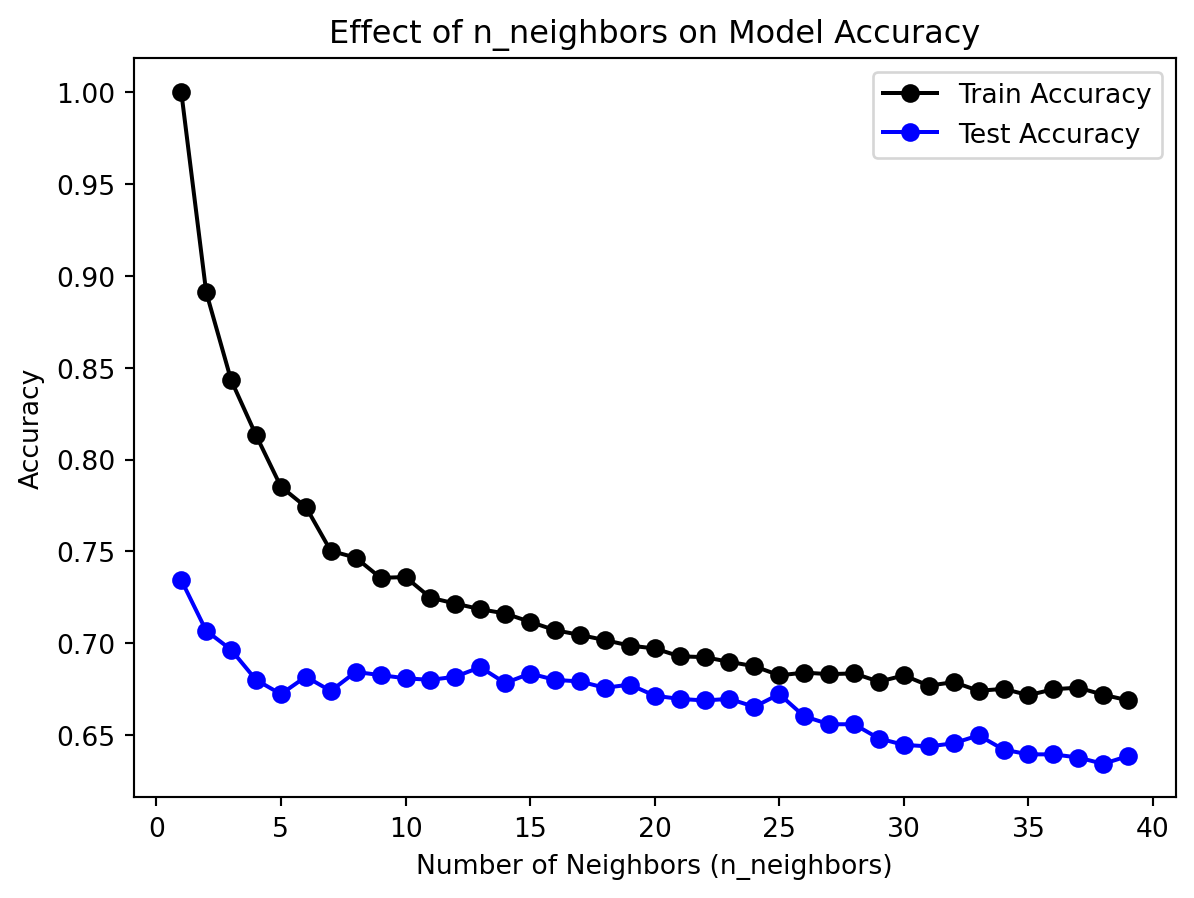
The default KNN model performs poorly on both the training and test data, with many misclassified samples. This may be due to inappropriate number of neighbors n_neighbors used in the default model. We will apply hyperparameter tuning to find the optimal KNN model that minimizes test error.
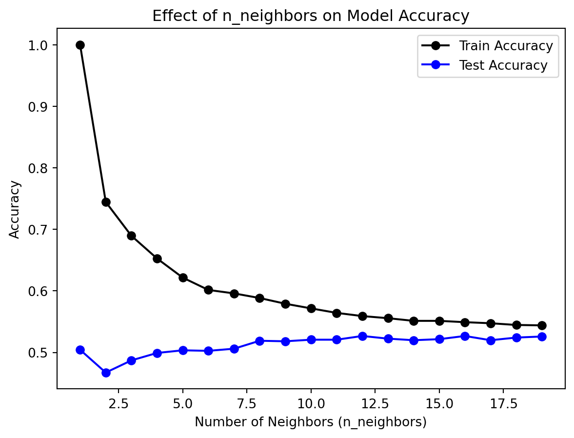
KNN Hyperparameter Tuning
In this section, we tune the number of neighbors n_neighbors for the KNN classification model to assess its impact on model performance.
def tuning_nneighbor(minn, maxn):# Range for n_neighbors neighbors_range =range(minn, maxn)# Lists to store train and test accuracies train_accuracies = [] test_accuracies = []# Loop through different n_neighbors valuesfor n in neighbors_range: model = KNeighborsClassifier(n_neighbors=n) model.fit(X_train, y_train)# Predictions for both train and test sets yp_train = model.predict(X_train) yp_test = model.predict(X_test)# Store accuracies train_accuracies.append(accuracy_score(y_train, yp_train)) test_accuracies.append(accuracy_score(y_test, yp_test))# Plotting the results plt.plot(neighbors_range, train_accuracies, color='black', label='Train Accuracy', marker='o') plt.plot(neighbors_range, test_accuracies, color='blue', label='Test Accuracy', marker='o') plt.xlabel('Number of Neighbors (n_neighbors)') plt.ylabel('Accuracy') plt.title('Effect of n_neighbors on Model Accuracy') plt.legend() plt.show()tuning_nneighbor(1, 40)
From the tuning results, we observe that the test accuracy scores are generally below 0.7, with the maximum at n_neighbors=1. This suggests that the best number of neighbors is 1. However, we know that in this case, the model will focus too much on local properties, leading to overfitting. Therefore, we conclude that KNN is not an ideal model for classification in our context. This could be due to KNN’s sensitivity to feature scaling. Since some features in our dataset are categorical (after one-hot encoding) and others are continuous, it is difficult to scale all features to the same range. As a result, features with different scales may negatively impact the model’s performance.
To address this issue, we will use Random Forest to explore non-linear relationships.
Random Forest Classification
Random Forest is also used for classification tasks. For classification tasks, it assigns the class label based on a majority vote from all the trees. In the context of classifying consumer complaints, Random Forest can effectively predict the category of a complaint based on a variety of features, such as product type, issue, company, sentiment score, and complaint length. The key advantage of using Random Forest is its ability to handle large datasets with many features and its robustness in dealing with both numerical and categorical data.
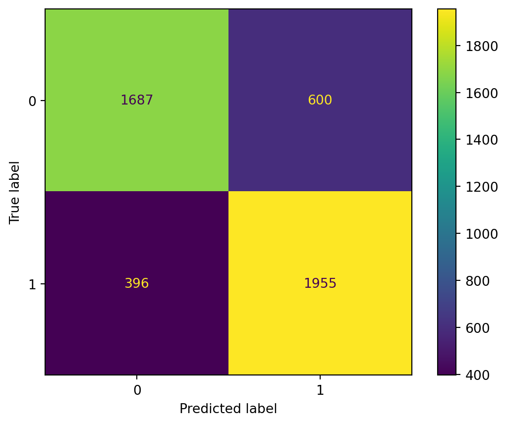
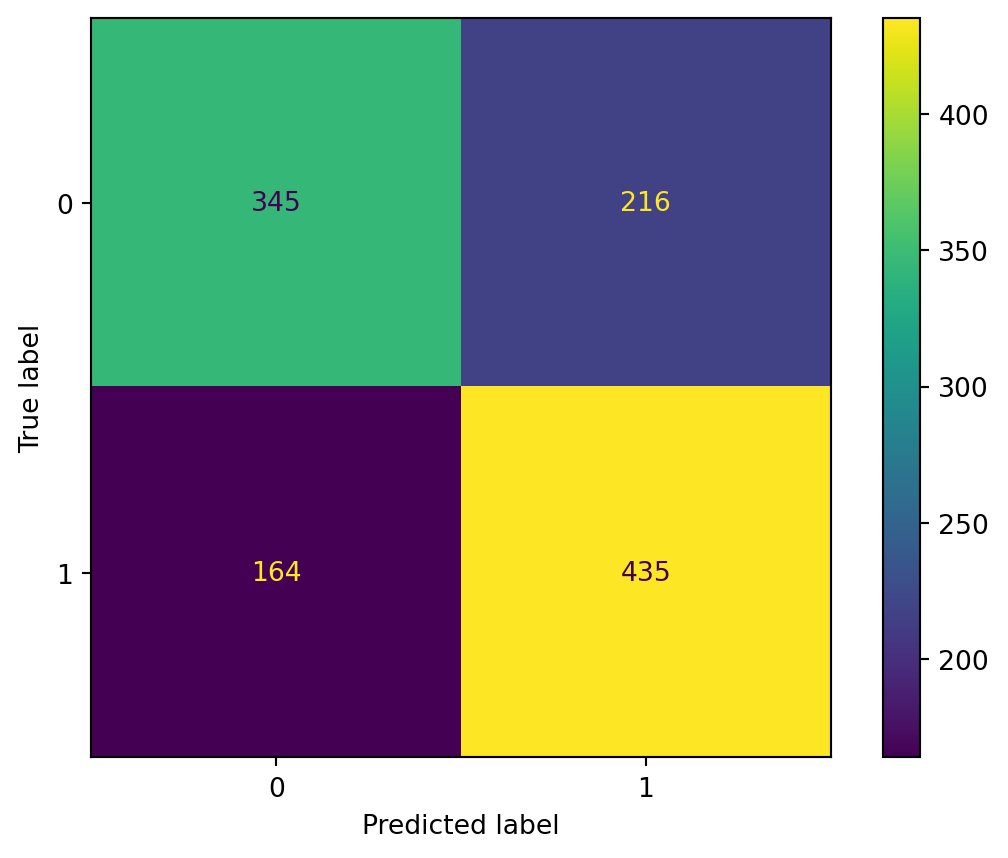
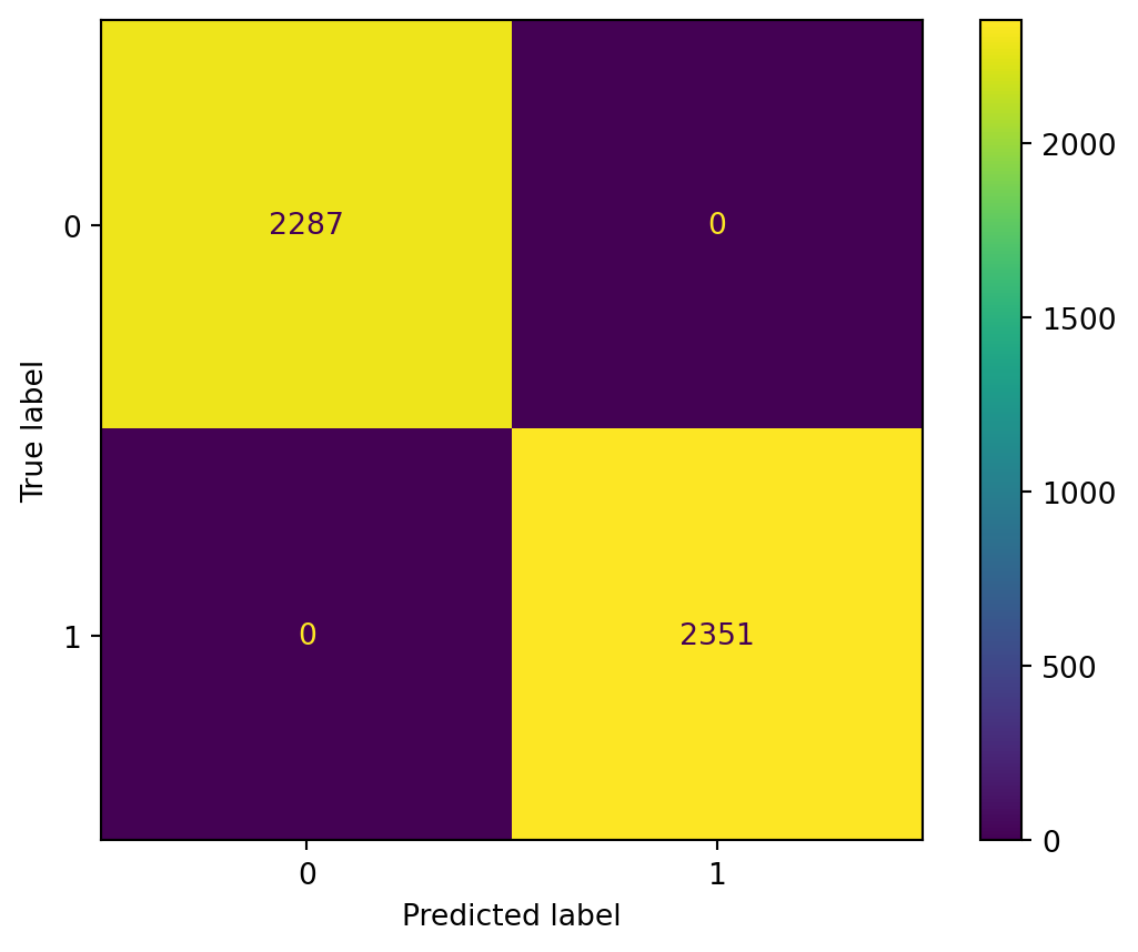
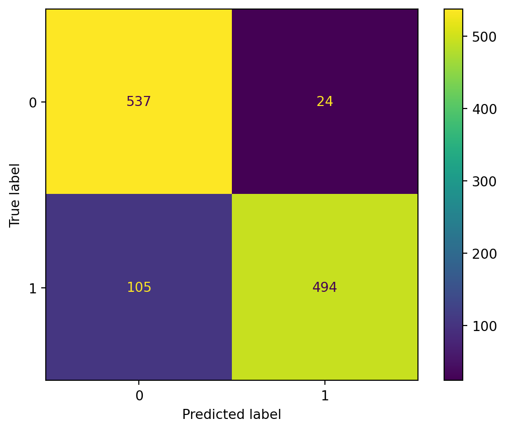
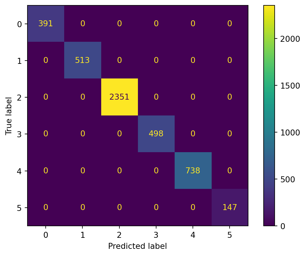
From the results, we can observe a strong performance from the Random Forest classifier. For the training data, the model achieves perfect accuracy, with an accuracy score of 1. The model correctly predicts all the labels within the training set, suggesting that it learns the relationships within the training data very well.
For the test data, the accuracy score is 0.88, which is still quite good. The model generalizes well to new, unseen data. Although this is slightly lower than the training accuracy, it is typical for a model to perform slightly worse on the test set due to the inherent variability and noise in real-world data.
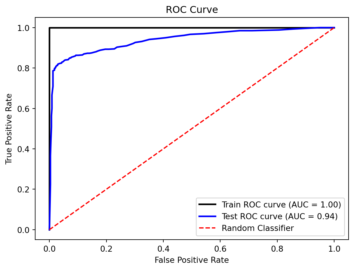
In addition to the accuracy, we can also assess the model’s performance through the ROC curve and the Area Under the Curve (AUC) score. For the training data, the ROC curve has an AUC score of 1, which is ideal and indicates that the model perfectly distinguishes between classes. For the test data, the AUC score is 0.94, which is still great and shows that the model maintains high classification power even when applied to unseen data.
Multi-class Classification
For multi-class classification, the target variable consists of six categories of complaints: Banking, Credit card, Credit reporting, Debt collection, Loan, and Money transfer. These categories are labeled from 0 to 5. The corresponding labels and their count values are shown below.
Other features, data preprocessing methods, and the train-test split method are the same as in the binary classification part.
from sklearn.preprocessing import LabelEncoder# Drop irrelevant columnsX = df.drop(columns=['Complaint_ID', 'Complaint', 'Tags', 'Product', 'Sub-product', 'Issue', 'Sub-issue','Date', 'Company Response', 'Company Public Response', 'cleaned_complaints','Category'])print(X.columns, end='\n\n')encoder = LabelEncoder()y = encoder.fit_transform(df['Category'])category_counts = df['Category'].value_counts()print("Original Categories and Corresponding Labels:")for i, category inenumerate(encoder.classes_):print("label", i, ":", category, ", count:", category_counts[category])# One-Hot Encoding for categorical columnscategorical_cols = X.select_dtypes(include=['object']).columnsX = pd.get_dummies(X, columns=categorical_cols, drop_first=True)# Split data into train and test setsX_train, X_test, y_train, y_test = train_test_split(X, y, test_size=0.2, random_state=50)
In addition to the confusion matrix and accuracy score introduced in the binary classification section, we use the Macro, Micro, and Weighted F1 scores to measure the performance of the multi-class classifier.
Macro F1 Score: This is the unweighted average of the F1 scores for each class. It treats all classes equally, regardless of their frequency. It is useful when we want to assess the model’s performance across all classes, especially when the classes are imbalanced.
Micro F1 Score: This calculates the F1 score globally by considering all true positives, false positives, and false negatives across all classes. It is useful when the class distribution is imbalanced, as it gives more weight to the smaller classes.
Weighted F1 Score: This is the average of the F1 scores for each class, weighted by the number of instances in each class. It accounts for the class imbalance, giving more importance to the classes with more samples.
def confusion_plot_multi(y_data, y_pred): cm = confusion_matrix(y_data, y_pred)print("ACCURACY:", accuracy_score(y_data, y_pred))# Macro and Micro F1 scores for multi-classprint("MACRO F1 SCORE:", f1_score(y_data, y_pred, average='macro'))print("MICRO F1 SCORE:", f1_score(y_data, y_pred, average='micro'))print("WEIGHTED F1 SCORE:", f1_score(y_data, y_pred, average='weighted'))print(cm) disp = ConfusionMatrixDisplay(confusion_matrix=cm) disp.plot() plt.show()def clas_evaluation_multi(y_train, y_test, yp_train, yp_test):print("------TRAINING------") confusion_plot_multi(y_train, yp_train)print("------TEST------") confusion_plot_multi(y_test, yp_test)
One-vs-Rest (OvR) Classification
One-vs-Rest (OvR) is a strategy for multi-class classification where a separate binary classifier is trained for each class. Each classifier learns to distinguish one class from all other classes. For each prediction, the model outputs the class with the highest score among all classifiers. This approach is simple and effective, especially for models like Logistic Regression.
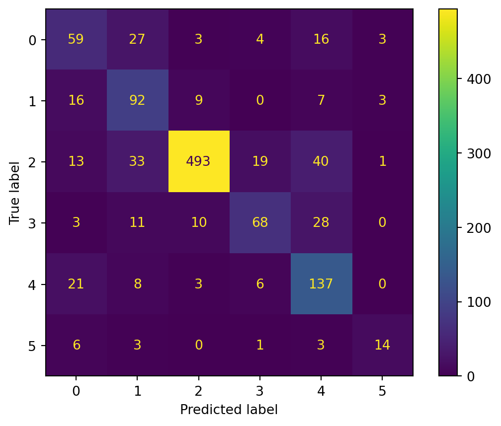
from sklearn.multiclass import OneVsRestClassifier# Create and train a Logistic Regression model wrapped in OneVsRestClassifiermodel = OneVsRestClassifier(LogisticRegression(max_iter=10000))model.fit(X_train, y_train)# Predictionsyp_train = model.predict(X_train)yp_test = model.predict(X_test)clas_evaluation_multi(y_train, y_test, yp_train, yp_test)
The model performs fairly well in both training and testing. The accuracy drop from the training set (0.78) to the test set (0.74) indicates some level of overfitting. The Macro F1 score drop from training (0.68) to testing (0.0.64) indicates that there may be more imbalanced performance across classes on the test set. Weighted F1 scores show that the model is somewhat biased towards the more frequent classes.
KNN Classification for Multi-class
Hyperparameter Tuning
tuning_nneighbor(1, 20)
From the tuning results, we observe that the test accuracy score is consistently low, around 0.5. Based on our earlier discussion in the binary classification section, we have decided to abandon the KNN model for this classification task.
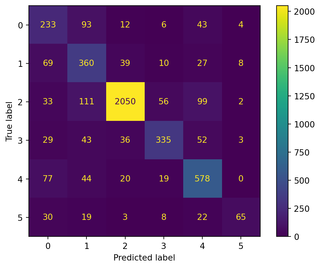
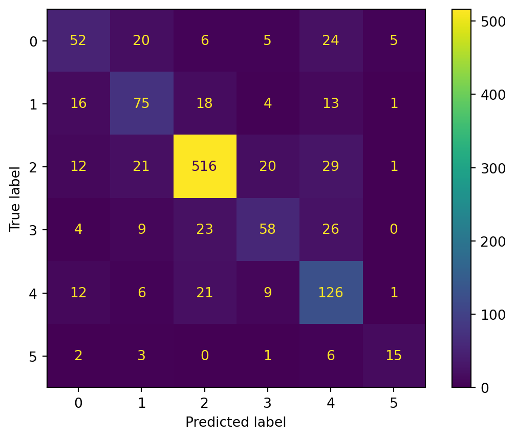
The Random Forest model performs perfectly on the training data, with an accuracy score and F1 scores of 1.0. This shows that the model has completely learned the training data. However, on the test data, both the accuracy and the weighted F1 score drop to 0.71. This suggests that the model is overfitting to the training data, as its performance is much lower on unseen data. The macro F1 score of 0.59 also shows that the model struggles with some smaller classes.
Conclusion for Classification Analysis
For binary classification, the Random Forest classifier outperforms the Logistic Regression model.
For multi-class classification, considering the imbalance in our dataset, we focus on the Weighted F1 score for the test dataset as the evaluation criterion. Based on this, we believe the One-vs-Rest model is the best choice. While the Random Forest model achieves perfect results on the training data, it may lead to undesired overfitting, making it less reliable for generalization.